Loan Amortization For Year-rest Installment Loan

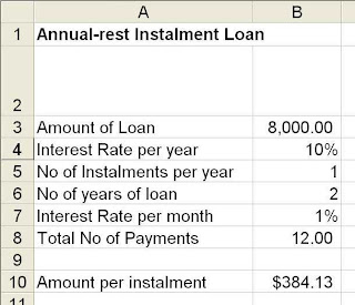
This blog will teach you how to work out a rough schedule for a yearly-rest installment loan. A yearly-rest loan is a loan where the principal amount is reduced on a yearly basis. To work out a schedule for this type of loan, you must first work out how much is the yearly installments and divide that by two. To do this, open a spreadsheet and do the following below. Remember to follow each step as it says or the formula will not work.

Suppose if you would like to apply for a two-year loan of $8,000 at 10% per annum. To work out the monthly installment amount:
1) In Cell A1, type " Annual-rest Installment Loan"
2) In A3, type "Amount of Loan".
3) In B1, type "8,000"
4) In A4, type "Interest Rate per year"
5) In B4, type "10%"
6) In A5, type "No. of Installments per year."
7) In B5, type "2"
8) In A6, type "No of years of loan"
9) In B6, type "2"
10) In A7, type "Interest rate per month"
11) In B7, type "=B4/12"
12) In A8, type "Total number of installments"
13) In B8, type "12"
14) In A10, type "Amount per installment ="
15) In B10 , type "=PMT(B4,B6,-B3,0,0)"

The amount that you would have to pay for the installment is $384.13 per month.

To work out the loan amortization schedule, in the same spreadsheet, do the following:
1) In D1, type "Loan Amortization Schedule"
2) In E2 , type "Principal at beginning of month"
3) In F2, type "Interest due at end of month"
4) In G2, type "Installment Payment"
5) In H2, type "Principal Repaid"
6) In D3, type "=1"
7) In E3, type "B3"
8) In F3, type "$B$7*E3". Copy this formula from F4 to F26
9) In G3, type "=B10"
10) In H3, type "0". Copy this value from H4 to H13 and H15 to H25
11) In H12, type " =SUM(G3:G14)-SUM(F3:F14)". Copy this formula to H26
12) In D4 to D26, type 2 all the way to 24
13) In E4, type "E3-H3". Copy this formula from E5 to E26
14) In G4, type "=G3" and copy this formula from G4 to G24

The final result will look something like this:

You may change the figures in B3, B4 and B6 to see how this schedule changes together with the monthly payments payable. Do remember to change the number of payments in column D to correspond with the number of years.

Disclaimer: Please note that aside from the schedule above, there might be other charges by the bank such as admin fee, processing fee etc. Do check with your bank officer or financial planner before making any decision to go ahead with any bank loans.